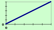
 Start
the simulation (by clicking on the Start button) and watch as the concentration
in the reservoir increases steadily.
 Work your way through the seven cases by clicking on the appropriate buttons and following the instructions that appear in this frame.
 Start
the simulation (by clicking on the Start button) and watch as the concentration
in the reservoir increases steadily.
Note that the lifetime (or residence time) is infinite since X is never removed from the reservoir. The lifetime represents the average time a pollutant molecule spends in the reservoir before being removed.
This is like turning on a tap and allowing a bath (with a plug in) to fill up.
When you have got the idea move on to the next case.
 Start
the simulation and watch as the concentration in the reservoir decreases
exponentially.
Note that the lifetime is constant and the rate of removal of X decreases as less X is left in the reservoir.
This is like pulling out the plug from a full bath (with both taps turned off) and letting it empty naturally.
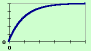 Start
the simulation and watch as the reservoir fills up to a constant level
(steady state).
Note that at steady state the rate of input and the rate of removal of X are the same.
This is like turning on a tap to try to fill a bath when you have forgotten to put a plug in the bath. The bath fills up a little but eventually the rate of removal becomes equal to the rate of input and the level in the bath reaches a steady value.
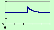 Run
the simulation until it reaches a steady state, then stop it.
Now increase the concentration of X to 110 (to simulate a release of pollutants) and re-start the simulation.
Note that the system gradually returns to its previous steady state.
This is like the sudden (effectively instantaneous) release of pollutants like one sees following a volcanic eruption or an explosion.
Note that the lifetime is not affected by the addition of more pollutants.
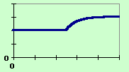 Run
the simulation until it reaches a steady state, then stop it.
Now increase the rate of input of X to 1.2 and re-start the simulation.
This is like the increased rate of emission of carbon dioxide that occured at the start of the Industrial Revolution.
Note that the lifetime is not affected by the increased rate of addition of pollutant.
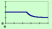 Run
the simulation until it reaches a steady state, then stop it.
Now increase the rate constant for the removal of X to 0.02 and re-start the simulation.
Note that the system quickly establishes a new steady state with a lower concentration of X than before and shorter lifetime.
This is like the effect that would be seen on the concentration of carbon dioxide in the atmosphere if a large area of new forest was planted to take CO2 out of the atmosphere.
Note that the lifetime has decreased as the rate of removal of pollutant has increased. Faster removal means a shorter residence time.
Run the simulation.
Note that it is already at steady state.
Now alter the rate of input to 2 ppm day-1 and the rate constant for removal to 0.02 day-1.
Run the simulation again and note that the system is still in a steady state but that the lifetime is now shorter. Repeat for values of 3 ppm day-1 and 0.03 day-1 etc.
For any system at steady state the rate of input is equal to the rate of removal. If both of these rates are low the lifetime (residence time) of the pollutant in the reservoir will be long but if both of these rates are high the lifetime of the pollutant in the reservoir will be short.